A Brief Report of the 2019 First Deep Time Data Science Workshop
May 28-31, Moscow, ID, USA
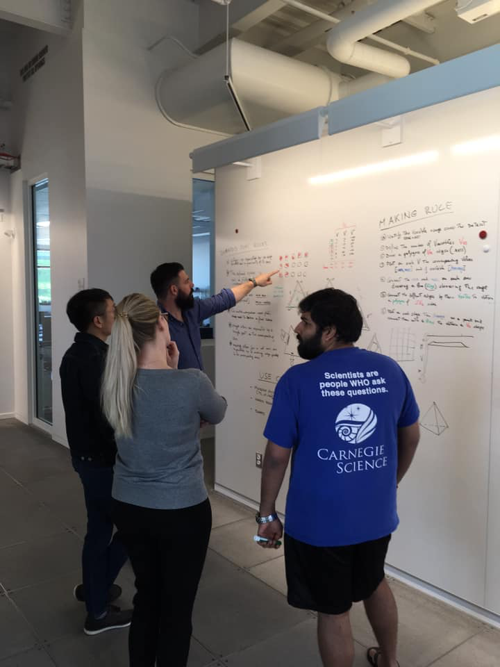
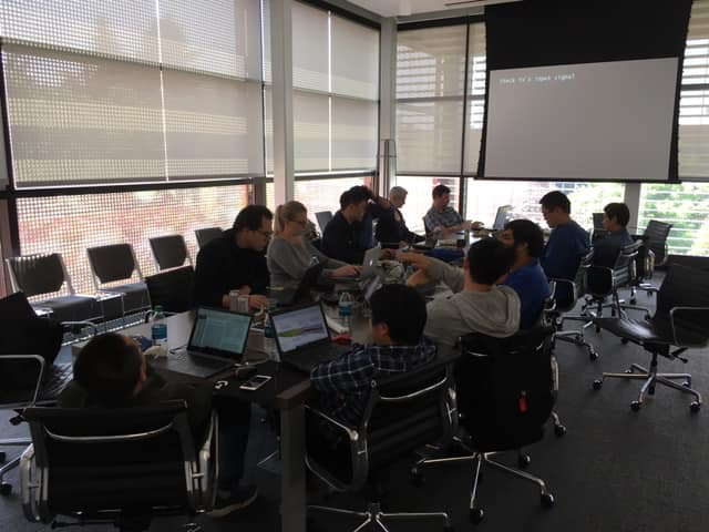
The topic Deep Time has drawn a lot of attention in geoscience and other disciplines. Several international initiatives, such as the 4D (Deep-time Data Driven Discovery) and DDE (Deep-time Digital Earth), are making rapid developments on research programs. With the emerging vast investment and broad participation, those initiatives will revolutionize global geoscience research in the next decades. As indicated in the introduction of both 4D and DDE, data will be the new driving force for geoscience. Data can be used in many ways, including both big and small data. The vast amount of data may even lead to a shift in the research paradigm, i.e. from the conventional hypothesis-guided research process to an exploratory and abductive process. This mini-workshop will be organized in an Agile style to reflect those changes and offer an opportunity for participants to learn new research methods. A few guiding questions and datasets will be provided prior to the workshop time, and we also encourage participants to bring their own datasets and questions. In the best way, they can also post their resources and needs to other participants in an earlier time. The structure of the workshop is flexible, and will include a) short lightning talks, b) presentations about dataset, questions and thoughts, c) datathon sessions in small groups, and d) short reports of datathon activities. Those activities will run through an iterative process till a satisfied result is achieved. Our goal is that, by the end of the workshop, each breakout group can envision or even already have a draft paper based on their work. Below is a short summary of the datathon work during the three-day period of the workshop.
1 Exploration between microbiology and data science
- Members: Donato Giovannelli, Chao Ma, Fang Huang
The work at the intersection between microbiology and data science included two different projects. In the first project, we worked to extract the concentration of the major elements composing standard microbiology growth media and look at their distribution across the tree of life. Extensive data cleaning and manipulation have been necessary to get the data in a suitable format to be analyzed, and linking the two different data resources required extensive coding performed both in R and Python. The two data resources used where the KOMODO growth media database (http://komodo.modelseed.org/default.htm) and the Silva Prokaryotic Type Strain phylogenetic tree based on the 16S rRNA gene (https://www.arb-silva.de/projects/living-tree/). The work carried out during the workshop has allowed to i) explore different clustering techniques to identify growth media that have similar composition, ii) explore the relative concentrations of trace elements in the growth media, and iii) explore the trace element distribution across the tree of life. tested clustering techniques included Self-Organizing Maps (SOM) and other unsupervised clustering techniques including nMDS and networks. the relative concentration of the different elements and their distribution across the tree of life were investigated with a combination of R and python tools and plotted using the phyloseq R package. The work carried out on this project will jump-start some of the downstream analyses, eventually leading to meet the project objective of obtaining a growth media-prediction tool.
At the same time, the group worked on a new type of visualization, aimed at presenting multivariate data across multiple sets to allow for quick visual comparison of the ranges associated with each variable. The work included the realization of a plan to roll out the first release of the visualization package as well as a number of use cases to present the new visualization technique to a broad interdisciplinary audience. The new visualization tool will be presented applied to data ranging from microbiology, geology, planetary science, and economy and should soon lead to a publication.
2 Mineral evolution map and data visualization
- Members: Marshall Ma, Dan Hummer, Xin Mou, Xiang Que, Shaunna Morrison, Bob Hazen
This small group has done two works in the past three days: 1) the initial prototype of a mineral evolution map; and 2) Element-mineral co-relationship data retrieval and visualization. Both works are based on the mineral evolution database that Josh and Alex are working on. They have added age attributes (first occurrence and last occurrence) to mineral species. The current database is organized by the mineral species of different elements.
In the first work, the designed mineral evolution map works in these steps: 1) Select a element (e.g., H) from a periodic table; 2) In the geologic time table, select a time concept (i.e. an early boundary and a late boundary); 3) Get all the H mineral species with first occurrence age inside the coverage of the selected time concept (This part can be updated to get all H mineral species with first occurrence age older than the late boundary of the selected time concept); 4) Calculate the paleo-coordinates of the selected mineral species records at the time of the late boundary of the time concept (because at that time they all exist); 5) Generate a paleogeographic map by using the late boundary of the time concept, and overlay the results of H mineral records on the map. There can be updates to this first work. For example, we can redesign the whole work to make it an animation (e.g. generate a H mineral species accumulation animation with an image for each 1 Ma). We can also do inclusion and exclusion of elements in the MED data retrieval, e.g. H minerals that also contain S, or H minerals without S.
In the second work, we retrieved the presence and absence data from element-mineral co-relationship data on the Mineral Evolution Database. A example of presence data: number of ‘O+H’ minerals that also contains S. An example of absence data: number of ‘O+H’ minerals that without S. Each data is a 72*72*72 Matrix. Dan will apply Chi-square test to the datasets to further see the impact of a third element on the mineral species of two other elements. Then this result can be visualized in Marshall’s 3D Klee diagram.
3 Application of Self-Organizing Map in clustering analysis of two use cases
- Members: Chao Ma, Shuang Zhang, Bob Hazen, Shaunna Morrison, Donato Giovannelli,
Self-organizing map (SOM) is a method of unsupervised data visualization and dimensionality reduction, introduced by Finish professor Teuvo Kohonen (Kohonenm 1997). It is a type of artificial neural network (ANN) with two layers: input and output layer, which utilizes the algorithm of competitive learning.
Pros of SOM:
- Intuitive way to visualize the mapping
- Relative simple algorithm and easy to interpret
- Predict new data fitting to the clustering
Cons of SOM:
- Difficult of representing too many properties in two dimensions
- Data must be numeric
This method was applied to two data sets in this workshop. One is a microbial media data set that needs to be clustered to investigate the types of media that is limiting the microbial culture. This data set is not well resolved by the SOM cause the data is not cleaned enough at the beginning to get a meaningful result through SOM. The other challenge is that data has a large number of dimensions (300+) and sparse (lots of zeros). Data is in cleaning process before next round SOM analysis after the workshop.
The second data set is pyrite data with contents of 12 elements aiming to be clustered to achieve a mineral natural kind classification. 9 clusters were grouped, but maybe not much meaningful according to Anirudh and Shaunna’s explanation in the aspects of minerology.
Conclusion: SOM can do clustering. Before doing SOM, data should be cleaned enough to meet the standards for SOM. SOM might do a better job for very large datasets. The difficult part of clustering algorithms is interpretation and verification. The choice of clustering methods are data specified. The workflow of SOM has been learned and constructed. It can be applied in future works of other data sets for dimensionality reduction and data visualization and clustering.
Reference:
T. Kohonen. Self-Organizing Maps. Springer-Verlag Berlin Heidelberg, 2nd edition, 1997.
4 Natural kind clustering of mineral species
- Data: Dan Gregory (UToronto) and Ross Large (UTasmania) Pyrite Data, Simone Runyon (UWyoming)
- Participants: Anirudh Prabhu, Fang Huang, Shuang Zhang, Shaunna Morrison, Bob Hazen, Drew Muscente, Chao Ma
Goal: Use cluster analysis to identify natural “types” of pyrite that correspond to unique formational environments. Based on the clustering results, we will classify the natural “type” and, therefore, predict the formational environment of pyrites of unknown origin.
Data Description:
Dan Gregory’s pyrite geochemistry database, including formational environment labels
Ross Large’s sedimentary pyrite geochemistry database
Simone Runyon’s tourmaline geochemistry database
Method:
We explored various clustering methods on the pyrite dataset from Dan Gregory. We found that model based clustering using the Mclust package in R performs a very robust model estimation. Many Gaussian mixture models were compared with various k-values for each clustering algorithm. The best results, evaluated using BIC and ICL metrics were produced by using VEV(ellipsoidal, equal shape) models with 9 clusters. These clusters when compared with deposit style of the samples showed interesting patterns. These patterns pose interesting research questions that can be pursued in future research. We have also assigned the cluster numbers from the Gaussian mixture models to train a random forest classifier. This model performed has an accuracy of 90.75%. And “accurately” identified groups in Ross Large’s pyrite dataset. We also performed cluster analysis on a tourmaline geochemistry database provided by Simone Runyon and found that the tourmalines segregate into 9 natural “types.”
Attendees:
- Shaunna Morrison, Carnegie Institute of Washington, Geophysical Lab
- Bob Hazen, Carnegie Institute of Washington, Geophysical Lab
- Drew Muscente, University of Texas, Austin
- Anirudh Prabhu, Rensselaer Polytechnic Institute
- Fang Huang, Rensselaer Polytechnic Institute
- Donato Giovannelli, University of Naples / Rutgers University
- Dan Hummer, Southern Illinois University
- Xin Mou, Lucid
- Shuang Zhang, Yale University
- Hanting Zhong, Chengdu University of Technology
- Anqing Chen, Chengdu University of Technology/ Purdue University
- Emily Forsberg, Geol., University of Idaho
- Leslie Baker, Geol., University of Idaho
- Terry Soule, CS, University of Idaho
- Marshall Ma, CS, University of Idaho
- Chao Ma, CS, University of Idaho
- Xiang Que, University of Idaho
Organizing Committee:
- Xiaogang (Marshall) Ma, University of Idaho
- Chao Ma, University of Idaho
- Leslie Baker, University of Idaho
- Emily Forsberg, University of Idaho
- Sue Branting, University of Idaho
- Arleen Furedy, University of Idaho
- Shaunna Morrison, Carnegie Institute of Washington, Geophysical Laboratory
- Anirudh Prabhu, Rensselaer Polytechnic Institute
- Fang Huang, Rensselaer Polytechnic Institute